How to Read a PostgreSQL EXPLAIN ANALYZE Plan Without Getting Lost
PostgreSQL execution plans may look intimidating, but they simply show how the database finds and processes your data. Using a real query over millions of rows, this guide explains the key terms and provides a simple checklist for spotting performance problems.

PostgreSQL execution plans can feel like a wall of technical language:
The good news is that you do not need to understand every number immediately.
Start with one simple question:
Where did PostgreSQL spend work to produce the final rows?
This guide uses a real query over millions of rows and explains the plan in plain language. By the end, you will have a repeatable checklist for reading your own plans.
The query
We want orders that use an International shipping method:
The database contains one million customers, one million synthetic shipping-method rows, and five million orders.
Here is the resulting plan:
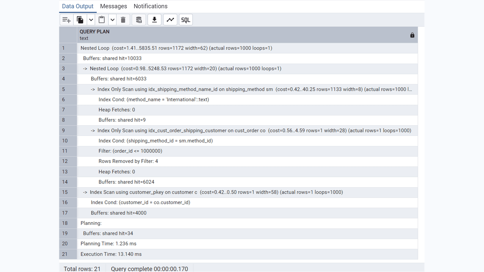
The plan returned 1,000 rows in 13.140 ms. That is already our first useful conclusion: this query is not slow.
What the EXPLAIN options mean
The query uses:
ANALYZE
Without ANALYZE, PostgreSQL only estimates what it would do.
With ANALYZE, PostgreSQL actually executes the query and reports real row counts and runtime:
Be careful when using it with INSERT, UPDATE, or DELETE: those statements really execute.
BUFFERS
This reports how PostgreSQL accessed data pages:
It helps distinguish memory activity from storage activity.
TIMING OFF
PostgreSQL still reports total execution time but avoids timing every individual row-processing operation. This reduces measurement overhead.
If you need per-node timing for diagnosis, run a separate plan without TIMING OFF:
SUMMARY ON
This prints the planning and execution summary at the bottom.
Where should you start?
Use two passes.
First, start at the bottom summary:
This tells you whether there is a performance problem worth investigating.
Second, read the indented data-producing nodes from the deepest level upward. Child nodes produce rows for their parent nodes.
For this plan, the execution story is:
Do not assume that PostgreSQL executed the SQL clauses from top to bottom. The optimizer is free to reorder joins and choose whichever access paths it estimates to be cheapest.
Step 1: find International shipping methods
The deepest starting node is:
In plain language:
Why Index Only Scan is good here
The index contains the filter column and the value required by the next step. PostgreSQL can answer this part using only the index.
Heap Fetches: 0 confirms that the main table was not visited.
Step 2: find orders for those methods
The next node is:
PostgreSQL takes each of the 1,000 International method IDs and performs an indexed order lookup.
The line:
means that this node ran 1,000 times and returned approximately one row per invocation.
Approximate total output:
PostgreSQL reports rows as an average per completed loop, and displayed values may be rounded. Multiplication gives an approximate total.
Rows removed by the filter
The plan says:
Approximately four rows were rejected per loop:
The index found orders using a method ID, then PostgreSQL applied:
That condition appears as a Filter, not an Index Cond, because order_id is an included column in the current index rather than a searchable key.
Understanding INCLUDE in an index
The order index is:
Think of the two groups differently:
PostgreSQL can navigate the index using the key columns. The included columns are payload: they can be returned from the index, but they are not used to navigate to a smaller range of index entries.
For example, this can use shipping_method_id as an index condition:
But this condition cannot use the included order_id as a search key in that index:
It becomes a filter after matching index entries are found.
A query-specific alternative would be:
That could allow both conditions to appear under Index Cond. Do not add it automatically: the current query is already fast, and every index adds storage and write-maintenance cost.
Step 3: combine methods and orders
The first parent node is:
A nested loop works like this:
Here:
Nested loops are not automatically bad. They work well when the outer side is reasonably small and the inner side has a fast index lookup.
They become suspicious when the outer side contains millions of rows and the inner operation is repeated millions of times.
The buffer total comes from the child operations:
Step 4: find customers
The customer node is:
PostgreSQL has 1,000 qualifying orders. It performs 1,000 customer primary-key lookups, finding one customer for each order.
It uses a regular Index Scan rather than Index Only Scan because the query needs:
Those values are in the customer table but not in the primary-key index.
Step 5: return the final rows
The top node is:
It combines qualifying orders with customer details and returns 1,000 rows.
The top buffer count includes its descendants:
Cost is not time
A node may show:
This means:
1.41: estimated startup cost5835.51: estimated total costrows=1172: estimated output rowswidth=62: estimated average row size in bytes
Cost is an internal planner unit, not milliseconds. Use it to understand why PostgreSQL preferred one candidate plan over another. Use Execution Time to measure the actual runtime.
Estimated versus actual rows
The top node says:
That estimate is reasonably close.
A dangerous mismatch looks like:
If PostgreSQL expects 10 rows but receives one million, it may choose a nested loop where a hash join would be more appropriate.
Possible causes include stale statistics, uneven data, related columns that are estimated independently, or expressions that are difficult to estimate.
Start by updating statistics:
Buffer terms in plain language
PostgreSQL stores table and index data in pages, normally 8 KB each.
shared hit
PostgreSQL found the requested pages in its shared memory cache.
shared read
PostgreSQL requested pages that were not already in shared buffers. The operating-system cache may still satisfy some reads, so this does not always mean a physical disk operation.
temp readandtemp written`
An operation used temporary storage, commonly because a sort or hash table did not fit in work_mem.
Your plan contains only shared hits. It was a warm-cache execution.
Heap fetches in plain language
The main PostgreSQL table storage is called the heap.
An index-only scan can still need to check the heap to confirm whether a row is visible to the current transaction:
That means PostgreSQL used the index but still visited the table many times.
Your plan shows:
The visibility map allowed PostgreSQL to trust the index entries without checking the table. VACUUM helps maintain this visibility information, although frequently updated tables may naturally require heap checks.
Sort and hash spills
A sort that fits in memory may show:
A sort that spills to temporary storage may show:
For a hash operation, multiple batches and temporary reads or writes can also indicate that the hash table did not fit in memory.
Possible responses include filtering earlier, adding an index that supplies the needed order, reducing the selected data, or carefully increasing session-level work_mem. Increasing work_mem globally can be dangerous because multiple operations and sessions may each receive their own allocation.
What a repeatedly executed SubPlan means
Consider this scalar correlated subquery:
Its plan may contain:
This means the internal lookup ran five million times and produced approximately one row per invocation.
It does not mean the final query returned five million rows. The subplan's result is used to test each outer order, and most orders may be rejected.
It also does not mean PostgreSQL sent five million separate SQL requests across the network. The database executor invoked that internal operation repeatedly inside one query execution.
A large loop count is important because even a small lookup becomes expensive when repeated millions of times.
Why the IN query has no SubPlan
The original condition is:
The inner query can be understood independently of the current order. PostgreSQL can convert the condition into semi-join logic:
The plan therefore integrates shipping_method into the main join tree instead of showing a separate SubPlan.
This is why an uncorrelated IN query and an explicit join can have similar performance. See the full comparison in PostgreSQL IN vs JOIN vs Correlated Subquery.
A nine-point execution-plan checklist
When you open a plan, check these points in order.
1. Execution time
Is the query actually slow? Do not optimize a 13 ms query just because the plan looks complicated.
2. Estimated versus actual rows
Large differences can cause unsuitable join and scan choices.
3. Rows multiplied by loops
means approximately five million internal row results from that node.
4. Scan type
Seq Scan: reads the table page by page; good when much of the table is needed.Index Scan: searches the index, then visits the table.Index Only Scan: may return everything directly from the index.
5. Rows removed by filters
Reading one million rows and rejecting 999,990 may reveal a missing or unusable index. Rejecting four rows per loop in a fast query may be harmless.
6. Buffers
shared hit: page found in PostgreSQL memoryshared read: page requested outside shared bufferstemp read/written: temporary storage activity
7. Heap fetches
For an index-only scan, zero heap fetches is ideal. A high count means PostgreSQL still visited the table.
8. Sort or hash spills
Look for external merge, Disk, multiple hash batches, and temporary reads or writes.
9. Subplans
Do not treat every subplan as bad. Check its loop count, rows, buffers, and time. A cheap one-time subplan is very different from a lookup repeated five million times.
The plan in one sentence
Our example plan says:
PostgreSQL found 1,000 International method IDs using an index, performed indexed order lookups, retained 1,000 qualifying orders, performed 1,000 customer primary-key lookups, and returned the result in 13.140 ms using cached pages.
That is an efficient plan.
Final takeaway
Do not begin by asking whether Nested Loop, Seq Scan, or SubPlan is always bad. Begin by asking:
An execution plan is a data-flow story. Start with the summary, then follow the deepest scans upward until you can explain how their rows became the final result.
